Local Indicators of Dispersion Scatterplot

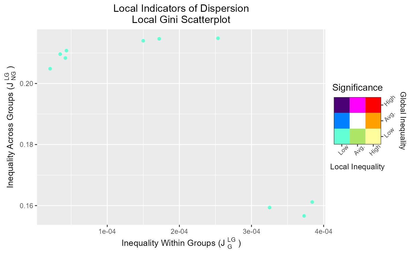
Plot the local group and non-group components of a local indicator of dispersion, colored by their inference-based class.

scatterLID(lid, inference, log.scale = FALSE, x.lim = NULL, y.lim = NULL)

colorLID(x = NULL, table = FALSE)

Arguments

lid

The list output of the LID function.

inference

The list output of the inferLID function.

log.scale

Logical. Should the axes be log-transformed? Default is FALSE. If TRUE, log transformation is log(1+x,10).

x.lim

One of NULL to determine the x-range automatically (the default), a numeric vector of length two providing the x boundaries, or a function that accepts the automatic boundaries and returns new limits (see scale_x_continuous).

y.lim

One of NULL to determine the y-range automatically (the default), a numeric vector of length two providing the y boundaries, or a function that accepts the automatic boundaries and returns new limits (see scale_y_continuous).

x

A character string or vector containing a LID significance class. Ignored if table = TRUE.

table

Logical. Should the function convert character strings of classes to hex codes of colors (table = FALSE, the default), or should it return the conversion table itself?

Value

A ggplot object with two elements---the LID Scatter plot and its scale.

Details

colorLID() acts as a function converting class names to the hex codes corresponding to the colors used by scatterLID when table = FALSE (the default), and returns the color table itself when table = FALSE.

Examples

# Generate dummy observations
x <- runif(10, 1, 100)

# Get distance matrix
dists <- dist(x)

# Get fuzzy weights considering 5 nearest neighbors based on 
# inverse square distance
weights <- makeWeights(dists, bw = 5, 
                       mode = 'adaptive', weighting = 'distance',
                       FUN = function(x) 1/x^2, minval = 0.1,
                       row.stand = 'fuzzy')
                       
# Obtain the 'local gini' value
lid <- LID(x, w = weights, index = 'gini', type = 'local')

# Infer whether values are significant relative to the spatial distribution
# of the neighbots
inference <- inferLID(lid, w = weights, ntrials = 100, pb = FALSE)

# Plot the inferences
scatterLID(lid, inference)